✒️ 论文公式总结
GIoU
$GIoU = IoU_{3d} - \frac{V_c - U}{V_c}$
其中,$V_c$代表能够包含两个框的最小立方体体积。$U$代表两个检测框的交集体积。
L2 distance
L2距离是简单的欧几里得距离。
$D_{\text{L2}}(\mathbf{x}, \mathbf{y}) = \sqrt{\sum_{i=1}^n (x_i - y_i)^2}$
Kalman Filter
Kalman滤波器是一种用于预测和估计动态系统的状态的滤波方法。下面是它在MOT中的常见形式。(CV/CA模型)
$$
\begin{align*}
x_{\text{pre}} &= A \cdot x \\
P_{\text{pre}} &= A \cdot P \cdot A^T + Q \\
K_k &= P_{\text{pre}} \cdot H^T / (H \cdot P_{\text{pre}} \cdot H^T + R) \\
x &= x_{\text{pre}} + K_k \cdot (z - H \cdot x_{\text{pre}}) \\
P &= (I - K_k \cdot H) \cdot P_{\text{pre}}
\end{align*}
$$
注意,filterpy库中的实现是略有不同的。对于最后一个公式,它进行了一定的修正。Extended Kalman Filter
扩展卡尔曼滤波器是基于普通卡尔曼滤波器的扩展,用于处理非线性系统。其原理是对模型进行泰勒一阶展开,从而处理非线性系统。下面是对常用非线性模型CTRV的扩展卡尔曼滤波器的数学公式。
$$
\begin{align*}
x_{pre} &=
\begin{bmatrix}
x_{pre} \\ y_{pre} \\ v_{pre} \\ \theta_{pre} \\ \omega_{pre}
\end{bmatrix} =
x +
\begin{bmatrix}
\frac{v}{\omega} \left( \sin(\omega \cdot \text{dt} + \theta) - \sin(\theta) \right) \\
\frac{v}{\omega} \left( \cos(\theta) - \cos(\omega \cdot \text{dt} + \theta) \right) \\
0 \\
\omega \cdot \text{dt} \\
0
\end{bmatrix} \\
P_{\text{pre}} &= J \cdot P \cdot J^T + Q \\
K_k &= P_{\text{pre}} \cdot J_h^T / (J_h \cdot P_{\text{pre}} \cdot J_h^T + R) \\
x &= x_{\text{pre}} + K_k \cdot (z - h(x_{\text{pre}})) \\
P &= (I - K_k \cdot J_h) \cdot P_{\text{pre}}
\end{align*}
$$
HOTA: A Higher Order Metric for Evaluating Multi-object Tracking
HOTA可以被视为三个IoU得分的组合。它将跟踪评估任务分为三个子任务(检测、关联和定位),并使用IoU(交并比)公式(也称为杰卡德指数)为每个子任务计算得分。
- 定位: 用于衡量追踪框和真实框之间的重合程度
- 检测: 衡量所有预测检测集合与所有真实检测集合之间的对齐程度
- 关联: 衡量预测关联集合与真实关联集合之间的对齐程度
最后综合考虑上面的三个方面,得到HOTA指标。(可能注意到没有LocA,因为这个指标内化在确定DetA和AssA中)
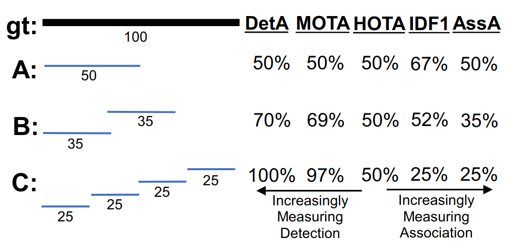
$$\mathrm{HOTA}_{\alpha} = \sqrt{\mathrm{DetA}_{\alpha} \cdot \mathrm{AssA}_{\alpha}}$$和其他指标的区别:
我们可以通过下面这个例子看到,在HOTA中关联和检测的权重几乎相同,而不是想MOTA中那样,检测的权重明显更高。我认为这是非常合理的。
KITTI坐标变换公式
$$ \mathbf{y} = \mathbf{P}_{rect}^{i} \cdot \mathbf{R}_{rect}^{0} \cdot \mathbf{T}_{velo}^{cam} \cdot \mathbf{x} $$推导过程:
- 点云齐次坐标(激光雷达坐标系)
- 激光雷达到相机的外参矩阵
- 相机坐标系矫正矩阵(畸变矫正)
注意,该步骤得到4*1列向量(x,y,z,1),当z小于0时,说明该点在相机后侧,应该被忽略。
- 相机内参矩阵(映射到i号相机图像)
- 图像坐标(齐次形式)
- 最终图像坐标(归一化后)
- 完整映射公式